Many of us are familiar with the VLOOKUP function. For those who are not, VLOOKUP is an Excel function to help you find values in a table or range. Microsoft Support has prepared a detailed explanation of the function at the following link:
https://support.microsoft.com/en-gb/office/vlookup-function-0bbc8083-26fe-4963-8ab8-93a18ad188a1
You will need to indicate the column number which you want the value to return. For example, the formula VLOOKUP(“12345”,A10:C20,2,TRUE) returns the value in the second column. In the current example, the value 2 is keyed in manually. Is there a way to further automate it?
Consider the following example.
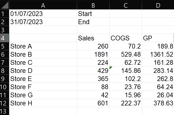
I am preparing a store performance report where I need to refer to some raw data downloaded from my accounting system. The raw data in the worksheet “RawData” and looks like this:

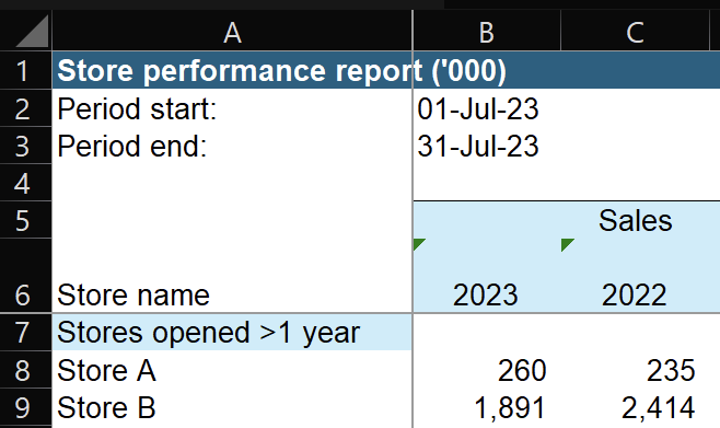
You want to reformat these data into a table in another worksheet which looks like this:

To organise the sales data for the stores into the table, I write the following formula in Cell B8:
=VLOOKUP(A8,RawData!$A$5:$D$12,2,FALSE)
In plain English, this formula first locates the row Store A (the value in cell A8) in cell range A5 to D12 of the RawData worksheet, and returns the data in the second column of that row which is the sales.
If I am to locate the COGS data of Store A, I can copy and paste the above formula and change the “2” to “3”, because the COGS data is in the third column. Can we automate the formula instead of manually changing the column number? Yes, if we use the formula function MATCH.
The MATCH function explanation from Microsoft Support is here:
https://support.microsoft.com/en-gb/office/match-function-e8dffd45-c762-47d6-bf89-533f4a37673a
It returns the relative position of an item in a range of cells. For example, if I write the following formula inside the RawData worksheet:
=MATCH(“Sales”,A4:D4,0)
It will return 2 because Sales is the second item in the cell range A4 to D4. Notice cell A4 is blank but still counted as the first item.
You may probably have guessed what I am going to do next:
=VLOOKUP($A8,RawData!$A$5:$D$12,MATCH($B$5,RawData!$A$4:$D$4,0),FALSE)
Hope this helps and good luck in the Excel journey.
P.S. One further question for you – in the formula above why I choose to use dollar signs differently for “A8”?